Plot Classification

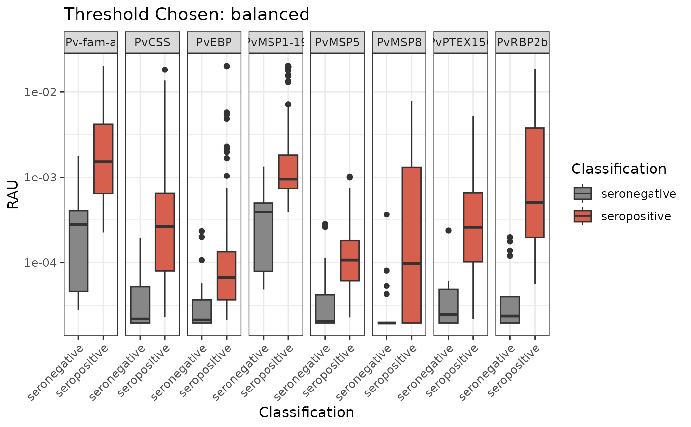
One example of data visualisation to detect the median and interquartile range of the RAU values per antigen for seropositive and seronegative individuals. Please note that the `classifyResults()` function must be run first.

Usage

plotBoxPlotClassification(all_classifications, selected_threshold)

Arguments

all_classifications

Data frame of `classifyResults()` for all sens_spec thresholds.

selected_threshold

String with the threshold.

Value

Box plots with RAU values for each protein stratified by classification (ggplot).

Author

Dionne Argyropoulos

Examples

# \donttest{

# Step 0: Load example raw data
your_raw_data <- c(
  system.file("extdata", "example_MAGPIX_plate1.csv", package = "SeroTrackR"),
  system.file("extdata", "example_MAGPIX_plate2.csv", package = "SeroTrackR")
)
your_plate_layout <- system.file(
  "extdata",
  "example_platelayout_1.xlsx",
  package = "SeroTrackR"
)

# Step 1: Read serology data and plate layout
sero_data  <- readSeroData(your_raw_data,"magpix")
#> PASS: File example_magpix_plate1.csv successfully validated.
#> PASS: File example_magpix_plate2.csv successfully validated.
plate_list <- readPlateLayout(your_plate_layout, sero_data)
#> Plate layouts correctly identified!

# Step 2: Process counts and perform quality control
qc_results <- runQC(sero_data, plate_list)

# Step 3: Convert MFI to RAU using ETH beads
mfi_to_rau <- MFItoRAU_Adj(
  sero_data    = sero_data,
  plate_list   = plate_list,
  qc_results   = qc_results
)
#> Joining with `by = join_by(antigen)`
#> Joining with `by = join_by(antigen)`
#> Joining with `by = join_by(antigen)`
#> Joining with `by = join_by(antigen)`
#> Joining with `by = join_by(antigen)`
#> Joining with `by = join_by(antigen)`

# Step 4: Define sens/spec thresholds
sens_spec_all <- c(
  "balanced", "85% sensitivity", "90% sensitivity", "95% sensitivity",
  "85% specificity", "90% specificity", "95% specificity"
)

# Step 5: Classify results across all thresholds
all_classifications <- purrr::map_dfr(sens_spec_all, ~{
  classifyResults(
    mfi_to_rau_output = mfi_to_rau,
    algorithm_type = "antibody_model",
    sens_spec = .x,
    qc_results = qc_results
  ) |>
  as.data.frame() |>
  dplyr::mutate(sens_spec = .x)
})

# Plot classification for a single threshold
plotBoxPlotClassification(all_classifications, "balanced")

# }